Lesson 5.9: Join Algorithms — How the Database Executes Joins
In previous lessons, we wrote SQL joins and focused on what data they return. But how does the database actually execute a join under the hood? Understanding the physical algorithms the engine uses is key to writing queries that perform well on large datasets.
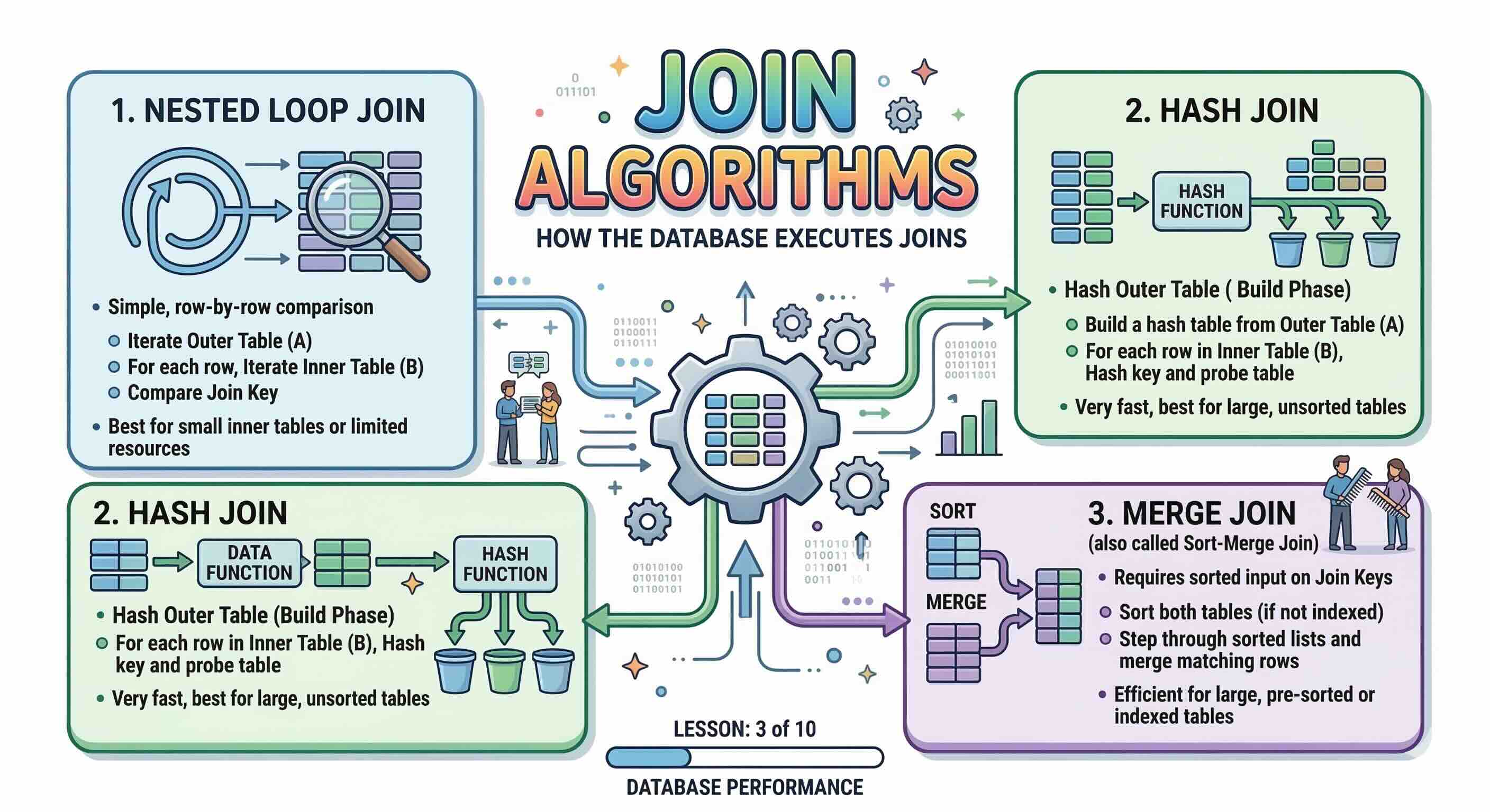
The three main join algorithms are:
- Nested Loop Join
- Hash Join
- Merge Join (also called Sort-Merge Join)
The query planner chooses one automatically based on table size, available indexes, and memory. We cannot force a specific algorithm in standard SQL, but understanding the trade-offs lets us write queries and create indexes that guide the planner toward the best choice.
1. Nested Loop Join
How It Works
The Nested Loop Join is the simplest algorithm. The database picks one table as the outer (driving) table and the other as the inner table. It then iterates over every row in the outer table and, for each row, searches the inner table for matches — essentially two nested for loops.
Conceptual pseudo-code:
for each row R1 in outer_table:
    for each row R2 in inner_table:
        if R1.key = R2.key:
            output(R1, R2)
When an index exists on the inner table's join column, the inner scan becomes a fast index lookup instead of a full table scan. This variant is called an Index Nested Loop Join and is one of the most efficient execution paths possible.
When the Planner Uses It
- The outer (driving) table is small.
- An index exists on the inner table's join column.
- The join uses a non-equality condition (
<,>,BETWEEN) — Hash Join and Merge Join require equality, so Nested Loop is the only option in this case.
Pros and Cons
| Nested Loop Join | |
|---|---|
| Pros | Works with any join condition, including range conditions |
| Extremely fast when the outer table is small and the inner table is indexed | |
| Low memory usage — no need to build auxiliary data structures | |
Starts returning the first result immediately (good for LIMIT queries) | |
| Cons | Very slow on large tables without indexes — O(N × M) in the worst case |
| Performance degrades rapidly as both table sizes grow |
2. Hash Join
How It Works
A Hash Join works in two phases:
- Build phase: The database reads the smaller table and builds an in-memory hash table keyed on the join column.
- Probe phase: The database scans the larger table and, for each row, looks up the hash table to find matching rows.
Conceptual pseudo-code:
-- Build phase
hash_table = {}
for each row R1 in smaller_table:
    hash_table[ hash(R1.key) ].append(R1)

-- Probe phase
for each row R2 in larger_table:
    for each match in hash_table[ hash(R2.key) ]:
        if R2.key = match.key:
            output(R2, match)
This gives an overall complexity of O(N + M) — linear in both table sizes — making it far more scalable than an unindexed Nested Loop Join.
When the Planner Uses It
- Joining two large tables on an equality condition.
- No useful index exists on the join column(s).
- Sufficient memory is available to hold the hash table (
work_memin PostgreSQL).
Pros and Cons
| Hash Join | |
|---|---|
| Pros | Very efficient for large-table joins — O(N + M) |
| Does not require indexes on the join columns | |
| Handles unsorted, unordered data well | |
| Cons | Requires an equality condition — cannot be used for range joins |
| Memory-intensive: if the hash table does not fit in RAM, it spills to disk (much slower) | |
| Higher startup cost — must build the hash table before returning any results |
Note: In PostgreSQL you can control the memory budget with the work_mem setting. Increasing it reduces the chance of expensive disk spills on large Hash Joins.
3. Merge Join (Sort-Merge Join)
How It Works
A Merge Join requires both input tables to be sorted on the join column. It then merges the two sorted streams simultaneously — very much like the final step of the classic Merge Sort algorithm — advancing a pointer through each stream to find matches.
Conceptual pseudo-code:
sort outer_table by key   -- skipped if an ordered index is used
sort inner_table by key   -- skipped if an ordered index is used

p1 = start of outer_table
p2 = start of inner_table

while not end of either stream:
    if outer[p1].key = inner[p2].key:
        output matching rows and advance both pointers
    elif outer[p1].key < inner[p2].key:
        advance p1
    else:
        advance p2
The critical optimisation: if the table can be scanned through an ordered index, the sort step is free and Merge Join becomes one of the most efficient algorithms available.
When the Planner Uses It
- Both tables are large and the join condition is equality.
- Both tables are already sorted, or both can be scanned via an ordered index.
- The query already requires
ORDER BYorGROUP BYon the join column (sorting happens anyway).
Pros and Cons
| Merge Join | |
|---|---|
| Pros | Very efficient for large tables when data is pre-sorted or an ordered index exists |
Produces output in sorted order, which can eliminate a later ORDER BY step | |
| Steady, predictable memory usage | |
| Cons | Requires an equality condition only |
| Expensive explicit sort step if neither table is pre-sorted and no index is available | |
| Less flexible than Hash Join when dealing with completely unsorted data |
4. Choosing the Right Algorithm
The query planner picks the algorithm automatically. You influence its decision indirectly by creating the right indexes and tuning memory settings.
| Scenario | Likely Algorithm |
|---|---|
| Small outer table + indexed inner table | Nested Loop Join |
| Two large tables, equality, no useful indexes | Hash Join |
| Two large tables, equality, both sorted / indexed in order | Merge Join |
Non-equality condition (<, >, BETWEEN) | Nested Loop Join (only option) |
Practical tips:
- Create indexes on frequently joined foreign key columns — this enables fast Index Nested Loop and Merge Joins.
- If a Hash Join is spilling to disk, consider increasing
work_memor reviewing whether the query can be restructured. - Use
EXPLAIN ANALYZEto inspect which algorithm the planner actually chose and how much time each step took:
EXPLAIN ANALYZE
SELECT a.first_name, a.last_name, f.title
FROM actor AS a
INNER JOIN film_actor AS fa ON a.actor_id = fa.actor_id
INNER JOIN film AS f ON fa.film_id = f.film_id;
Look for keywords like Hash Join, Merge Join, or Nested Loop in the output plan to identify the chosen algorithm and its cost.
Key Takeaways from This Lesson
- Nested Loop Join iterates rows in nested loops — fast for small tables with supporting indexes, very slow for large unindexed tables; the only algorithm that supports non-equality conditions.
- Hash Join builds an in-memory hash table from the smaller table and probes it — efficient for large unindexed tables joined on equality, but memory-intensive.
- Merge Join reads two pre-sorted streams simultaneously — ideal when data is already in order (e.g. via an index) and the join is on equality; produces results in sorted order as a bonus.
- All three algorithms support equality joins; only Nested Loop also supports range conditions.
- You influence the planner's choice through indexes, memory settings (
work_mem), and query structure — not by specifying the algorithm in SQL. - Always use
EXPLAIN ANALYZEto verify which algorithm is actually being used and where the time is being spent.